


By Ganesh Hegde, Director of Data Science and AI Strategy at KETOS, Inc.
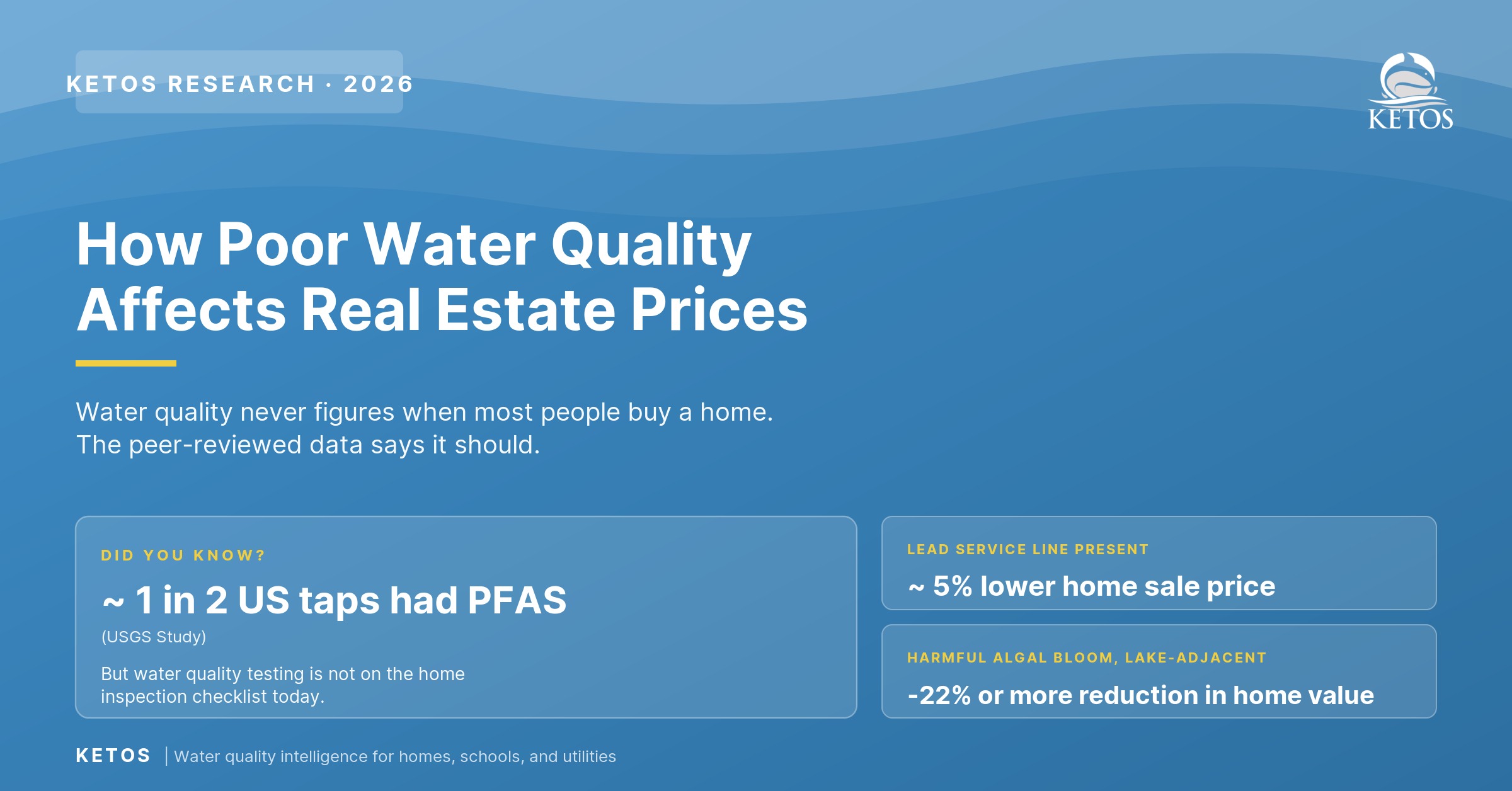
When most people buy or sell a home, water quality never comes up. The standard home inspection covers structural and mechanical systems and closes with a pest report. None of it includes a chemical test of the water coming out of the tap, which is treated as a problem someone else has already solved. For roughly half of US homes, that turns out to be wrong.
In 2023, the U.S. Geological Survey published the largest random-sample study of US tap water to date. It detected PFAS, the family of synthetic compounds linked to cancer, thyroid disease, and immune suppression, in approximately 45% of US tap water samples, roughly half of all taps tested. The EPA’s 2024 National Primary Drinking Water Regulation set enforceable limits on six PFAS compounds, but water utilities have until 2027 to begin notifying customers about detections and until 2029 to bring systems into full compliance. The Consumer Confidence Report your utility sends today is not yet required to disclose PFAS at the new regulatory threshold.
The implication for buyers and sellers transacting between now and 2029 is direct. Roughly half of the homes changing hands in the United States are served by water that may not meet the standard their homes will eventually be measured against, and no one is required to disclose it until 2029. Water quality testing is not part of the standard home inspection package today. Given what the research shows about the impact on the people living in the home, both their health and their home value, it should be. Treat it the way you treat the termite inspection and the sewer scope: a non-optional step in due diligence that buyers should request and sellers should volunteer.
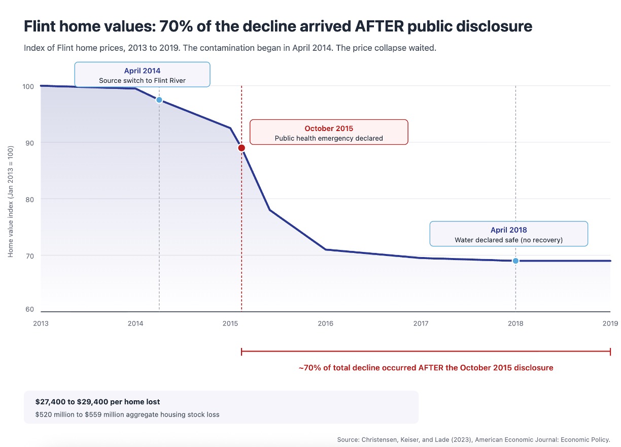
When disclosure finally does arrive, the economic evidence catches up to the cognitive gap fast. In April 2014, the city of Flint, Michigan, switched its drinking water source from Detroit’s distribution system to the Flint River. Lead concentrations at the tap began climbing almost immediately. But Flint’s home values did not. Most of the housing market damage waited for October 2015, when public health officials issued the emergency declarations that brought the lead-in-water story to national attention. Roughly 70% of Flint’s home value decline arrived after that disclosure, not after the contamination began (Christensen, Keiser, and Lade, 2023).
On declaration day, what had changed was the buyer’s information set, not the water chemistry. By the time a homeowner reads about a water quality issue in their service area, the price effect is already moving. By the time they list, it is already priced in.
This pattern, that home values respond to disclosure rather than to molecules, runs through the peer-reviewed literature on water quality and real estate. This article reviews that evidence across four areas: lead in drinking water, PFAS contamination, drinking water service reliability, and surface water quality at waterfront properties. Every estimate below is research-derived, every range is tied to its source, and every dollar figure is a capitalization estimate, not an appraisal.
Quick reference: how water quality moves home prices
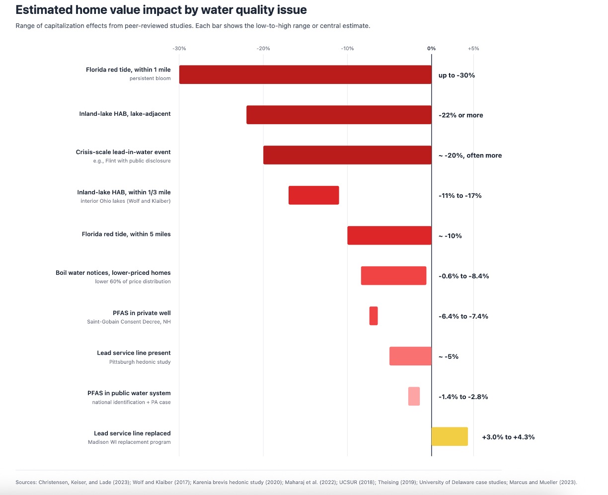
The table below aggregates the strongest peer-reviewed and industry-grade estimates in the literature. Each row identifies the contamination type, the size of the home value impact, the underlying study, and the geography it covers. Local conditions, market timing, and individual home characteristics will shift any specific case. The direction and approximate magnitude are well established.
| Water quality issue | Estimated impact on home value | Source | Geography |
|---|---|---|---|
| Crisis-scale lead-in-water event with public disclosure | Roughly $27,400 to $29,400 per home; 20% or more for many neighborhoods | Christensen, Keiser, and Lade (2023) | Flint, MI |
| Lead service line still present | About 5% lower sale price, roughly $9,700 | UCSUR (2018) | Pittsburgh, PA |
| Lead service line replaced | 3.0% to 4.3% price lift, about $5,914 at median home price | Theising (2019) | Madison, WI |
| PFAS detected in public water system | 1.4% to 2.8% lower | Marcus and Mueller (2023); Pennsylvania UDel case | National; Bucks and Montgomery Counties, PA |
| PFAS in private well | 6.4% to 7.4% lower | New Hampshire UDel case | Saint-Gobain Consent Decree region, NH |
| Recurring boil water notices, lower 60% of price distribution | 0.6% to 8.4% lower | Maharaj et al. (2022) | Marion County, WV |
| Inland-lake harmful algal bloom, within one-third mile | 11% to 17% lower | Wolf and Klaiber (2017) | Ohio (Grand Lake St. Marys, Buckeye Lake) |
| Inland-lake harmful algal bloom, lake-adjacent | 22% or more lower | Wolf and Klaiber (2017) | Ohio |
| Florida red tide within five miles, persistent bloom | About 10% lower | Karenia brevis hedonic study (2020) | Southwest Florida |
| Florida red tide within one mile, persistent bloom | Up to 30% lower | Karenia brevis hedonic study (2020) | Southwest Florida |
| Lake clarity gain, positive scenario | About $3,681 per 0.1 m Secchi gain at average lakefront home | Mamun et al. (2023), PNAS | National lakefront |
These ranges are research-derived capitalization estimates, not appraisals. Use them as benchmarks, not as price determinations for a specific home.
Quick-reference checklist: water quality and home value
Six items each for sellers and buyers, drawn from the research below. Save, share, or print.
For sellers
- Pull your local Consumer Confidence Report and document any violations in the past five years.
- Test for lead using a first-draw and flush sample from the kitchen tap; document service line material from city records if available. KELP’s home water test kit covers lead alongside 30+ contaminants with EPA-certified methodology.
- Test for PFAS using EPA Method 533 or 537.1, especially on a private well or in any service area with known historical AFFF use, manufacturing operations, or military installations.
- On a private well, also test for nitrate, total coliform, and arsenic at minimum.
- Document every result in writing and disclose proactively in the listing rather than at inspection.
- If a recurring boil water notice or violation affected your area, note the history and any remediation taken.
For buyers
- Request a recent water test as part of your inspection package, not as an afterthought. KELP’s mail-in home water test kit uses EPA-certified methodology and is designed for residential due diligence.
- Pull the address’s Consumer Confidence Report and review the past five years of violations and treatment changes.
- If the home has a private well, request the well log, recent test results, and any prior remediation records.
- For PFAS-suspected areas, check the PFAS Grade for the zip code before commissioning the specific test.
- If a lead service line is present, expect roughly a 5% lower sale price or budget for replacement (about $5,000 to $10,000 in most metros).
- If contamination is detected: walk, renegotiate the price to reflect remediation cost, or condition closing on completed remediation.
Estimated home value impact by water quality issue. Sources: Christensen, Keiser, and Lade (2023); Wolf and Klaiber (2017); Karenia brevis hedonic study (2020); Maharaj et al. (2022); UCSUR (2018); Theising (2019); University of Delaware case studies.
Why disclosure drives capitalization
Christensen, Keiser, and Lade (2023), publishing in the American Economic Journal: Economic Policy, ran a difference-in-differences analysis on Flint home sales matched to comparable cities. The April 2014 switch to the Flint River corroded distribution-system lead pipes and raised lead concentrations at the tap almost immediately. Prices began softening, but the larger move came later. After October 2015, when Genesee County and city officials issued public health declarations and the lead-in-water story became national news, the bulk of the decline arrived. Flint’s housing stock lost between $520 and $559 million in value relative to the counterfactual. On a per-home basis, the decline ran $27,400 to $29,400. The crisis dropped many neighborhood prices by 20% or more.
The persistence of the effect is the part that should worry sellers. Even after Flint completed lead service line replacements and the federal government spent more than $400 million on remediation, home prices remained depressed through August 2019, more than 16 months after the water was declared safe to drink.
Why does the timing matter so much? Because by the October 2015 declaration date, the contamination had already been ongoing for 18 months. The chemistry of the water did not change on declaration day. The buyer’s information set did. Lenders, appraisers, inspectors, and prospective buyers all calibrated their decisions to publicly known facts. Disclosure was the price-moving event.
The same dynamic appears in the PFAS literature. Marcus and Mueller (2023) found that media coverage intensity, not measured contamination level alone, scaled with the size of the home value effect. Two homes with similar PFAS detections could see different price effects depending on how loud the local media coverage was. The implication for sellers is direct. Pre-listing testing is value-preserving because it converts a buyer-side surprise into a seller-side data point you can frame and address. The implication for buyers is also direct. The contamination at any given address may already be present, with the disclosure event still ahead. Future regulatory developments, including the EPA’s 2024 PFAS National Primary Drinking Water Regulation and ongoing Lead and Copper Rule Improvements implementation, will produce more disclosure events on a defined timeline.
Morckel and Rybarczyk (2022) surveyed Flint homeowners directly and added the human shape to the econometrics. A majority believed the crisis hurt their property values. More than half wanted to leave but felt unable to sell. About one in five had considered abandoning their homes. The dollar number from the regression carries a corresponding loss of mobility, optimism, and trust.
Concerned about contaminants in your water?
Get water testing from KETOS KELP using EPA-certified methodology, results you can trust, backed by real data.
Order a Water Test →Lead in drinking water
Crisis-scale events: what Flint actually cost homeowners
Flint is the most rigorously studied lead-in-water event in the United States, which is part of why its headline numbers anchor so much of this article. The Christensen, Keiser, and Lade (2023) analysis used a difference-in-differences design comparing Flint’s housing market with a synthetic control of comparable cities, then traced the effect through secondary mortgage market data and migration patterns. The aggregate housing stock loss was $520 to $559 million. The per-home loss was $27,400 to $29,400.
What made Flint particularly severe was the combination of three factors: a source switch that produced contamination, a regulatory failure to apply corrosion control, and the long disclosure lag between the start of the contamination in April 2014 and the public health declarations in October 2015. The longer the disclosure lag, the larger the eventual price correction tends to be, because by the time buyers learn, the perceived reliability of the local water system is already severely damaged.
Morckel and Rybarczyk (2022) added the second-order effects from a resident survey. A majority of Flint homeowners believed the crisis hurt their property values. More than half wanted to leave the city but felt they could not sell. About one in five had considered abandoning their homes outright. When a market loses confidence in a place, mobility freezes alongside prices.
Lead service lines without a crisis
The quieter, more universal story is about lead service lines themselves, not crisis events. Lead service lines (LSLs) are present in roughly 6 to 9 million US homes by EPA estimate, with the highest concentrations in older Northeastern and Midwestern cities. They affect home values whether or not a Flint-style disclosure event has occurred.
The University Center for Social and Urban Research at the University of Pittsburgh (2018) studied this directly. Their hedonic regression on Pittsburgh single-family sales found that homes with lead laterals sold for about 5% less on average (p ≈ 0.079). The average dollar reduction was $9,700, ranging from about $6,500 for two-bedroom homes to $13,000 for four-bedroom homes. Pittsburgh had not experienced a Flint-style crisis at the time of the study. Buyers were already pricing in the presence of lead, and the policy environment around the federal Lead and Copper Rule was already shifting.
Theising (2019), publishing in Environmental and Resource Economics, ran the same question from the opposite direction. Madison, Wisconsin, was the first US city to complete a universal LSL replacement program, which gave Theising a 16-year panel of property transactions and an unusually clean policy variation to identify the effect. After replacement, treated homes saw price lifts of 3.0% to 4.3%, equal to about $5,914 at the 2000 median assessed home price. The implied returns on remediation were striking. The combination of public and private replacement costs delivered an average return greater than 75%. The private cost alone, averaging $1,340, returned more than 300% in capitalization.
The two studies cohere. A still-present lead lateral discounts the home by roughly 5%. A replaced lateral lifts the home by roughly 3 to 4%. The total swing is on the order of 8% of home value, enough to cover the cost of replacement many times over. Theising flagged an equity dimension worth keeping in view: older homes with LSLs are disproportionately rented, so price lifts can pass through to renters as higher rent over time.
Lead service line replacement creates a roughly 8% swing in home value, large enough to cover replacement costs many times over. Sources: UCSUR Pittsburgh (2018); Theising (2019).
What schools and operators should know
The institutional and school audience belongs in a separate cluster anchored to KETOS SHIELD continuous monitoring, but a brief mention is appropriate for readers whose interest is professional or whose home is near a school with a known testing flag.
State-level school water testing programs have proliferated since 2017. Most states use a 15 ppb action level for lead in school drinking water, while a handful use considerably stricter thresholds: 5 ppb in California, 4 ppb in Vermont, 2 ppb in Illinois. When a school exceeds its state’s action level, parents are notified and the result becomes part of the public record.
The disclosure-timing insight from Christensen, Keiser, and Lade (2023) applies at the neighborhood level when a school discloses a positive lead test. The market reads the disclosure as a signal about the broader water system, even when the immediate fix is at the school’s own taps. KETOS continuous monitoring at Goddard School New Braunfels detected lead at 0.228 ppb across 140 days and nine locations, well below any state action level. That kind of proactive instrumentation is the institutional analog of a homeowner’s pre-listing test: it converts a disclosure event from a surprise into a data point that can be framed and addressed. For the institutional perspective on continuous water monitoring and lead-in-water testing in schools, utilities, and buildings, see our 2026 buyer’s guide on lead-in-water testing services, the methodology-first companion to this article.
PFAS and forever chemicals
PFAS, the synthetic class better known as forever chemicals, have moved from a niche environmental concern to a national regulatory priority over the past decade. The home value research has caught up. For the chemistry and health background, see our forever chemicals primer. Below is the property value evidence.
The national picture
Marcus and Mueller (2023), in NBER Working Paper 31731 and forthcoming in the Journal of Environmental Economics and Management, is the cleanest national identification we have on PFAS and home prices. Their difference-in-differences design used the EPA’s third Unregulated Contaminant Monitoring Rule (UCMR3), which required testing for several PFAS compounds at thousands of US public water systems between 2013 and 2015. Detection events provided a natural experiment, and the subsequent media coverage provided a measurable disclosure pulse.
Marcus and Mueller found that media coverage of PFAS detections produced statistically significant decreases in property values for affected homes, with effect size scaling with coverage intensity rather than with measured contamination level alone. Two homes with similar PFAS detection levels could see different price effects depending on how loud the local coverage was. The identification matches the pattern in Flint. Disclosure drives capitalization, not exposure.
The EPA’s National Primary Drinking Water Regulation for PFAS, finalized in April 2024, set enforceable Maximum Contaminant Levels for six PFAS compounds. Public water systems have until 2027 to comply with monitoring requirements and until 2029 to comply with treatment requirements where MCLs are exceeded. The regulatory schedule means the next several years will produce a wave of PFAS detection disclosures across the country, each one creating the kind of disclosure pulse that Marcus and Mueller found drives home value decline. The timing of those disclosures is broadly predictable from the schedule, but the specific service areas that will see them are not.
Public water system contamination, the Pennsylvania case
A University of Delaware case study examined PFAS impacts in Bucks and Montgomery Counties, Pennsylvania, where former military aviation operations contaminated public groundwater. The study analyzed 157,817 single-family transactions from 2010 through 2022 using a difference-in-differences hedonic.
Average property values within affected public water system service areas dropped 2.8% relative to comparable homes outside those service areas. The geographic pattern is typical of PFAS plumes: contamination concentrates near specific historical use sites, in this case the former Naval Air Station Joint Reserve Base Willow Grove and the former Naval Air Warfare Center Warminster, both legacy AFFF firefighting foam users. Adjacent communities with separate water systems generally did not see the same effect. The Pennsylvania case is broadly representative of what happens when PFAS contamination is identified in a public water system: a few percentage points off home value, geographically concentrated, persistent over time.
Private well users carry the heaviest burden
Private well users carry a markedly larger price effect than public water system users. A second University of Delaware case study, focused on the Saint-Gobain Consent Decree region of New Hampshire, ran a hedonic difference-in-differences specifically on private well households in Merrimack and surrounding towns.
Sale prices for homes on PFAS-contaminated private wells fell 6.4% to 7.4% from 2016 forward versus matched controls. The effect was roughly two to three times larger than the public water system effect found in Pennsylvania.
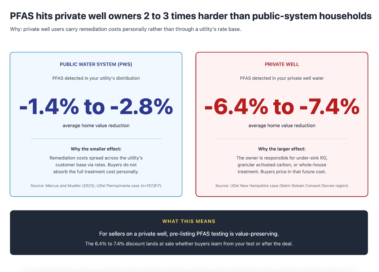
PFAS hits private well owners 2 to 3 times harder than public-system households. Sources: Marcus and Mueller (2023); University of Delaware Pennsylvania and New Hampshire case studies.
Private well users carry remediation costs personally rather than through a utility’s rate base. A buyer purchasing a private well home with a known PFAS detection is buying both the contamination and the bill for the under-sink reverse osmosis system, the granular activated carbon filter, or the whole-house treatment that the situation may require. The discount they negotiate reflects that future cost transparently.
This finding has direct practical implications. For sellers on a private well, pre-listing PFAS testing converts a buyer-side surprise into a seller-side data point. The 6.4% to 7.4% range applies whether buyers learn from your test or after the deal. For buyers, a recent PFAS test belongs in the inspection package alongside the well log and recent nitrate and coliform results. EPA Methods 533 and 537.1 are the relevant testing standards for PFAS in drinking water (see our practical guide on how to test water for PFAS for sample collection and method comparison). KELP uses these EPA-certified methodologies.
Test your home’s water with KELP.
Service reliability and routine violations
Boil water notices and the regressive burden
Boil water notices (BWNs) are the most common water service disruption affecting American homes. The federal Safe Drinking Water Act delegates BWN issuance to state primacy agencies and individual public water systems, which means coverage and frequency vary widely across the country. In rural and lower-income service areas, recurring BWNs are routine.
Maharaj, Collins, and colleagues (2022), publishing in Ecological Economics, used a spatial hedonic price model on 1,985 property transactions in Marion County, West Virginia, between 2012 and 2017. The county had an unusual data advantage: detailed records of BWN events combined with property sale data over a five-year window.
The findings are uneven across the price distribution. For properties in the lower 60% of the price distribution, a BWN paired with a one-day water disruption produced sale price declines of 0.6% to 8.4%. For properties at the 70th percentile and above, the effect was statistically indistinguishable from zero. Aggregated across the county, where most properties experienced repeated BWNs, the authors estimated that residential values likely declined by 1% to 10%.
Drinking water service reliability functions as a regressive tax on home value, concentrating the loss in the lower 60% of the price distribution while leaving more expensive homes substantially unaffected. For utilities, that asymmetry means investments in source water protection, treatment redundancy, and continuous monitoring deliver outsized benefits in the communities most economically exposed to service failures.
SDWIS violations and Superfund cleanups
Beyond BWNs, the broader question of how routine drinking water violations affect home prices runs through two interconnected literatures: the Consumer Confidence Report regime under the Safe Drinking Water Act, and the Superfund cleanup literature.
The 2024 Consumer Confidence Report Rule revisions take effect for reports due July 1, 2027. They require community water systems serving more than 10,000 people to publish twice-yearly water quality reports, surfacing violation history that would otherwise be invisible to buyers. The buyer-friendly nature of CCRs means that improvements over time, or worsenings, become a public record that attaches to a community’s housing market.
The Superfund cleanup literature offers a useful counterweight to anyone tempted to overclaim how much remediation moves prices. Greenstone and Gallagher (2008), publishing in the Quarterly Journal of Economics, used a regression discontinuity comparing the first 400 NPL-listed Superfund sites with 290 sites that narrowly missed listing. They found cleanup associated with economically small and statistically insignificant changes in tract-median housing values. The headline took hold in the literature as a skeptical reference point.
A follow-up by Gamper-Rabindran and Timmins, using more granular data, found large positive cleanup effects at the lower deciles of within-tract sale prices: 20.9% at the 10th percentile, 16.3% at the median, and 12.2% at the 60th percentile. The two studies disagree on the magnitude but agree on the direction: cleanups matter most where homes are cheapest. The pattern matches the Maharaj BWN finding. Drinking water service quality is a regressive amenity, and improvements compound at the lower end of the market.
How to read a Consumer Confidence Report
Every public water system serving more than 10,000 people publishes an annual Consumer Confidence Report, available on the utility’s website or through the EPA SDWIS Federal Reports Search. Look for the violation history table, any contaminants detected at or above the Maximum Contaminant Level, and recent treatment process changes. A clean CCR is a buyer’s ally and a seller’s documentation. A CCR with recurring violations or recent treatment changes warrants a closer look at the home itself.
Surface water quality and waterfront homes
Inland-lake harmful algal blooms
Wolf and Klaiber (2017), publishing in Ecological Economics, is the foundational study on harmful algal blooms (HABs) and inland-lake property values. They ran a multi-lake hedonic across six Ohio counties from 2009 through 2015, focused on Grand Lake St. Marys and Buckeye Lake, both of which suffered persistent cyanobacteria blooms during the study period.
For homes within roughly one-third of a mile of either lake, capitalization losses ran 11% to 17%. For lake-adjacent homes, the loss exceeded 22%. An Ohio State University release tied to the paper estimated about $152 million in lost property value to Ohio homeowners over the six-year window. (That figure aggregates effects on the two interior Ohio lakes the paper studied, not Lake Erie. Some secondary coverage conflates the two.)
Toxic algal blooms degrade the recreational value of waterfront property: the swimming, fishing, and aesthetic amenities that drive lakefront premiums in the first place. When the bloom becomes a recurring summer phenomenon, the discount becomes structural rather than seasonal.
Lake Erie
Lake Erie is the largest and most studied freshwater HAB system in the United States. Bingham, Sinha, and Lupi (2016), in an AAEA conference paper, used a repeat sales model on Lake Erie lakefront properties to control for unobserved characteristics of individual homes that have been a known weakness in cross-sectional hedonic studies of HAB effects.
Their finding: a one microgram per liter reduction in chlorophyll-a is associated with about a 2% home price increase, with effect decaying rapidly with distance from shore. Stated in reverse, a one microgram per liter increase in chlorophyll-a is associated with about a 1.7% to 2% decrease, or roughly $2,205 at the relevant baseline home price.
The Lake Erie pattern reinforces the inland-lake findings. HAB severity translates directly into lakefront premium erosion. Treatments that reduce nutrient loading from agricultural runoff in the Maumee River watershed, the dominant nutrient source for the western basin, would produce direct property value benefits in the affected counties.
Florida red tide
Saltwater HABs follow a similar pattern with even larger magnitude effects. Karenia brevis red tide events striking Southwest Florida coastal communities have been studied through hedonic event models that compare sale prices during persistent blooms with sale prices in matched coastal areas not affected by the bloom in the same period.
Within five miles of the coast, prices decline about 10% during a persistent bloom. Within one mile of the coast, prices fall as much as 30% versus comparable homes in unaffected counties in the same month (Karenia brevis hedonic study, 2020). A 2020 Journal of Real Estate Finance and Economics paper used wind direction as an instrument to identify exogenous variation in shore exposure, confirming that the effect is causal rather than spuriously correlated with other coastal disamenities.
Coastal premiums are large in absolute dollar terms, which means even modest percentage declines translate into meaningful absolute losses. Buyers and lenders in red tide-prone communities have started incorporating bloom history into pricing decisions, much as flood risk has become a routine consideration in hurricane-prone areas.
The upside: water clarity raises waterfront value
The same hedonic methods that quantify HAB damage also quantify the upside of water quality improvements. Mamun, Kreller, Polasky, and colleagues (2023), publishing in PNAS, ran the largest national study of lakefront property values and water quality to date, drawing on roughly 674,000 transactions near 1,632 lakes. The methodology combined Zillow ZTRAX sales data with the LAGOS-NE database and the federal Water Quality Portal.
A 0.1-meter increase in Secchi depth, the standard field measure of water clarity, is worth about $3,681 at the average lakefront home within 100 meters of shore. Regional estimates from prior studies cluster around the same value, ranging from about $850 in Northern Maine to $5,540 in Orange County, Florida.
Two earlier papers anchor the same finding in different contexts. Leggett and Bockstael (2000), in the Journal of Environmental Economics and Management, studied 1,183 Maryland Chesapeake Bayfront transactions and found that a change of 100 fecal coliform per 100 mL was associated with a 1.5% change in price, with mean absolute effects of $5,114 to $9,824 in 1997 dollars. Walsh, Griffiths, Guignet, and Klemick (2017), in an EPA NCEE working paper, followed up across 14 Chesapeake Bay counties: a one-foot improvement in Secchi depth raises housing prices by about $9,600, decreases time on market by 19.7 days, and reduces seller holding costs by about $1,280.
The waterfront market reads water quality continuously, in both directions. Pollution events erode lakefront premiums quickly. Source water protection and clarity improvements raise them just as durably. For waterfront communities, watershed-scale water quality investment shows up directly in lakefront property values, with measurable returns on the order of those documented above.
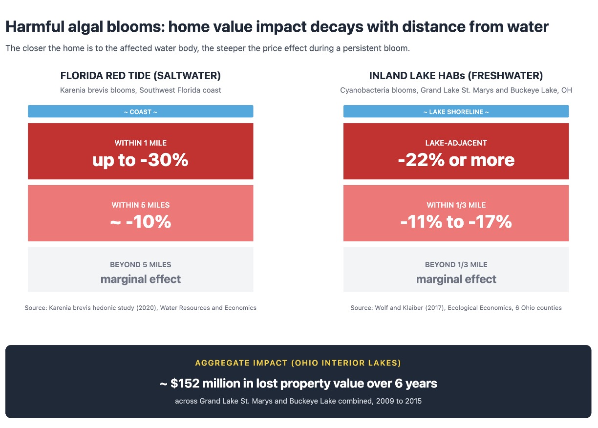
Harmful algal bloom impact decays with distance from the affected water body. Sources: Karenia brevis hedonic study (2020); Wolf and Klaiber (2017).
How buyers actually use this information
The disclosure-driven price effect documented across the studies above raises a practical question: do buyers actually use water quality information when it is available, or do they ignore it?
The cleanest evidence comes from outside the water quality literature. Redfin ran a controlled experiment with 17.5 million users, displaying flood risk scores from First Street Foundation to half the audience and not to the other half. Among users looking at homes with severe or extreme flood risk, those exposed to the risk scores made offers on homes with 50% less risk than the control group (Redfin / First Street). Disclosure shifted behavior measurably even when not legally required.
The 2024 NAR Profile of Home Buyers and Sellers showed that 83% of recent buyers ranked heating and cooling costs as at least somewhat important in their home selection. Environmental and operating-cost considerations are now mainstream buyer criteria. Water quality belongs in that frame, particularly as buyers in jurisdictions with strong disclosure regimes become accustomed to seeing the data.
The asymmetry between markets with strong disclosure and markets without it is where the dynamic concentrates. State-level water quality disclosure laws vary widely. Most states require disclosure of known contamination on private wells at sale, but enforcement and definitions vary. Public water system Consumer Confidence Reports are federally required but rarely enter the listing or inspection process by default. The result is that buyer attention to water quality is mostly demand-driven rather than regulatorily forced. A seller who provides a recent test pre-listing is providing information the market values, regardless of whether the law requires it.
What to do before listing or buying
If you would not skip the termite inspection or the sewer scope, do not skip a water test. PFAS now shows up in roughly half of US tap water samples, and federal compliance with the new limits is not required until 2029. The absence of a public complaint is not the same as the absence of a problem. What follows is the practical playbook for sellers, buyers, and institutional operators.
The seller and buyer guidance below is packaged as a one-page PDF you can share with your realtor or inspector: Download “The Water Quality Blind Spot in Real Estate” checklist.
For sellers
The economic logic for sellers in markets where contamination is plausible is direct. The 6.4% to 7.4% private well PFAS discount, or the 2.8% public water system PFAS discount, lands at sale whether or not you have a documented test in hand. Pre-listing testing converts a buyer-side surprise into a seller-side data point you can frame and address.
The minimum useful pre-listing water test for residential sale spans several categories:
- Lead. A first-draw and flush sample from the kitchen tap, plus documentation of service line material from city records if available.
- PFAS. EPA Method 533 or 537.1, particularly important on private wells and in any service area with known historical AFFF use, manufacturing operations, or military installations.
- Private wells. Nitrate, total coliform, and arsenic at minimum, with iron, manganese, and pH for informational purposes.
- All properties. A check of the local Consumer Confidence Report for any recent violation history.
Document the results and disclose them proactively. Buyers respond more favorably to a transparent test result than to silence followed by inspection-stage discovery.
For buyers
Request a recent water test as part of the inspection package. Ask specifically about lead, PFAS where relevant to the location, nitrate where the home is on a private well, and any boil water notice history in the past five years. Pull the public water system’s Consumer Confidence Report for the address and look for violations during that window. For a quick view of PFAS risk in the area before commissioning a specific test, check the PFAS Grade for the zip code. If the home has a private well, ask for the well log and recent test results. If anything looks off, the options are familiar: walk, renegotiate the price to reflect the cost of remediation, or condition closing on completed remediation.
For schools, facilities, and operators
Continuous monitoring is the institutional analog of pre-listing testing. The disclosure-driven home value effect applies at the neighborhood level when a school discloses a positive lead test or when a public water system reports a violation. The economic argument for proactive instrumentation is the same on the institutional side: convert disclosure events from surprises into framed data points. For the institutional perspective, see our 2026 guide to lead-in-water testing services for schools, utilities, and buildings.
Test your home’s water before you list. KELP delivers EPA-certified methodology water testing in clear, defensible formats that buyers, inspectors, and lenders recognize.
Frequently asked questions
Should buyers test water like they test for termites?
Yes. Water quality testing belongs in the standard due diligence package alongside the structural inspection, termite report, and sewer scope. The U.S. Geological Survey detected PFAS in roughly 45% of US tap water samples in a 2023 nationwide study, and water utilities have until 2029 to be in full compliance with the EPA’s 2024 PFAS standards. Buyers transacting between now and 2029 cannot assume the absence of a public complaint means the absence of a problem. Sellers benefit from the same logic in reverse: a pre-listing water test removes a buyer-side surprise that would otherwise reduce sale price at inspection.
Does poor water quality lower home value?
Yes. The peer-reviewed evidence is consistent across contamination types. Confirmed lead-in-water events with public disclosure can lower per-home values by $27,400 to $29,400 (Christensen, Keiser, and Lade, 2023). PFAS detections reduce home values by 1.4% to 2.8% in public water systems and 6.4% to 7.4% on contaminated private wells (Marcus and Mueller, 2023). Inland-lake harmful algal blooms reduce lake-adjacent home values by 22% or more (Wolf and Klaiber, 2017).
By how much does PFAS contamination lower home value?
Public water system contamination reduces home values by an average of 1.4% to 2.8% (Marcus and Mueller, 2023). Private wells contaminated with PFAS see larger reductions, in the range of 6.4% to 7.4%, because owners carry remediation costs personally rather than through a utility’s rate base.
Do lead pipes affect home value?
Yes. Pittsburgh-area homes with lead service lines sold for about 5% less than comparable homes without them (UCSUR, 2018). Madison, Wisconsin, homes that completed lead service line replacement saw price lifts of 3.0% to 4.3% (Theising, 2019).
Should I test my water before buying a home?
Yes. A recent water test should be part of any home inspection package. For private wells, EPA Method 533 or 537.1 for PFAS, plus standard tests for lead, nitrate, and bacterial contamination. For public water systems, look up the address’s Consumer Confidence Report and review the past five years of violation history.
Does a boil water notice affect home value?
Yes, particularly for lower-priced homes. In Marion County, West Virginia, properties in the bottom 60% of the price distribution saw sale price declines of 0.6% to 8.4% (Maharaj et al., 2022). For homes in the top 30%, the effect was statistically indistinguishable from zero.
Are lakefront homes affected by harmful algal blooms?
Substantially. Inland-lake homes within one-third of a mile of a HAB-affected lake see capitalization losses of 11% to 17%; lake-adjacent homes see losses exceeding 22%. On the Florida coast, persistent Karenia brevis red tide blooms drop prices about 10% within five miles and up to 30% within one mile.
Where can I find my city’s water quality report?
Every community water system serving more than 10,000 people publishes an annual Consumer Confidence Report, usually on the utility’s website. The EPA SDWIS Federal Reports Search is an authoritative national lookup.
Methodology and sources
This article draws on peer-reviewed economics literature, federal data sources, and industry practitioner work compiled in a research brief that supports each numerical estimate above.
Three reminders apply when using these numbers. First, every estimate is a research-derived range, not an appraisal of any specific property. Second, geography and timing matter: a Madison-derived effect does not transfer cleanly to Phoenix, and a 2017 estimate may not capture 2026 market conditions. Third, capitalization studies measure average effects across many transactions; individual cases vary widely.
